十分钟读懂旋转编码（RoPE）

LLaMA、GLM 模型采用。

线性变换与旋转矩阵

旋转矩阵是一类特殊的线性变换矩阵。

有一类特殊的线性变换，叫做正交变换（其对应的矩阵称为正交矩阵）。这类变换的一个核心特性就是保角性，即变换前后任意两个向量之间的夹角保持不变。最常见的例子就是旋转矩阵。同时大小保持不变。

绝大多数线性变换都不具备保角性。它们会拉伸、压缩、剪切空间，从而改变角度。

位置编码

Transformer Architecture: The Positional Encoding - Amirhossein Kazemnejad's Blog

这篇文章介绍了为什么需要位置编码：(9 封私信 / 75 条消息) 一文读懂Transformer模型的位置编码 - 知乎

主要原因： Transformer 模型本身不具备像 RNN 那样的学习词序信息的能力，需要主动将词序信息喂给模型。

简单想一想，很远之前的一个 the 和我们将要 decode 的这个 token 前面的一个 the 位置是不一样的，对于下一个 token 的贡献也不应该是一样的。但是如果我们不加入位置编码，这两个位置的 the 对于下一个 token 的 attention 值（$QK^T$）是一样的，也就是我们需要投入相同的注意力，这是明显不合理的。

当然，没有像 RNN 一样的位置信息引入了另外一个好处，就是我们可以并行处理所有的 token，而 RNN 只能一个一个地处理，这极大地加快了 Transformer 结构的处理速度，是成也萧何，败也萧何。

简单想想：

我们能想出来两种方法：

1. 让所有的 token 的位置编码等间距散落在 $[0,1]$ 区间，有以下两个问题：
   • 不同的句子长度，区间内每一个步长是不一样的；
2. 1, 2, 3 这么一直排下去给每一个 token：
   • 值可能会很大，对于神经网络学习很不利；
   • 可能学习的时候长度比推理的长度短，导致没有学习到。

对编码的要求：

1. 每一个位置有一个唯一编码；
2. 两个位置之间的 step 应该是固定的，不应该和句子的长度有关；
3. 能够泛化到更长的句子；
4. 不能是随机的，必须是确定的。

初始的位置编码是如何实现的？

首先，这种编码不是单一的一个数值，而是包含句子中特定位置信息的 $d$ 维向量（和词向量一个维度，这是为了方便后面直接加到词向量上面，让词向量也带上了位置信息）。

给定一个长度为 $n$ 的输入 token 序列， $t$ 表示 token 在序列中的位置，$\overrightarrow{p_t} \in \mathbb{R}^d$ 用来表示 $t$ 这个位置的位置向量（p = position）。可见我们需要一个函数 $f: \mathbb{N}\rightarrow \mathbb{R}_d$ 来将位置映射到向量，定义如下：

\[\begin{array}{c} \overrightarrow{p_t}^{(i)}=f(t)^{(i)}:=\left\{\begin{array}{ll} {\sin \left(\omega_k \cdot t\right),} & {\text { if } i=2 k} \\ {\cos \left(\omega_k \cdot t\right),} & {\text { if } i=2 k+1} \end{array}\right. \tag{1} \end{array}\]

其中：

\[\tag{2} \omega_k=\frac{1}{10000^{2 k / d}}\]

注意 $i$ 表示这个向量里面的第 $i$ 个元素。分成了基数和偶数的情况。

\[\begin{array}{c} \overrightarrow{p_t}=\left[ \begin{array}{c} {\sin (\omega_1 \cdot t)} \\ {\cos (\omega_1 \cdot t)} \\ {\sin (\omega_2 \cdot t)} \\ {\cos (\omega_2 \cdot t)} \\ {\vdots} \\ {\sin (\omega_{d / 2} \cdot t)} \\ {\cos (\omega_{d / 2} \cdot t)} \end{array} \right] \\ \end{array}\] \[\begin{align} 0: \ \ \ \ \color{orange}{\texttt{0}} \ \ \color{green}{\texttt{0}} \ \ \color{blue}{\texttt{0}} \ \ \color{red}{\texttt{0}} & & 8: \ \ \ \ \color{orange}{\texttt{1}} \ \ \color{green}{\texttt{0}} \ \ \color{blue}{\texttt{0}} \ \ \color{red}{\texttt{0}} \\ 1: \ \ \ \ \color{orange}{\texttt{0}} \ \ \color{green}{\texttt{0}} \ \ \color{blue}{\texttt{0}} \ \ \color{red}{\texttt{1}} & & 9: \ \ \ \ \color{orange}{\texttt{1}} \ \ \color{green}{\texttt{0}} \ \ \color{blue}{\texttt{0}} \ \ \color{red}{\texttt{1}} \\ 2: \ \ \ \ \color{orange}{\texttt{0}} \ \ \color{green}{\texttt{0}} \ \ \color{blue}{\texttt{1}} \ \ \color{red}{\texttt{0}} & & 10: \ \ \ \ \color{orange}{\texttt{1}} \ \ \color{green}{\texttt{0}} \ \ \color{blue}{\texttt{1}} \ \ \color{red}{\texttt{0}} \\ 3: \ \ \ \ \color{orange}{\texttt{0}} \ \ \color{green}{\texttt{0}} \ \ \color{blue}{\texttt{1}} \ \ \color{red}{\texttt{1}} & & 11: \ \ \ \ \color{orange}{\texttt{1}} \ \ \color{green}{\texttt{0}} \ \ \color{blue}{\texttt{1}} \ \ \color{red}{\texttt{1}} \\ 4: \ \ \ \ \color{orange}{\texttt{0}} \ \ \color{green}{\texttt{1}} \ \ \color{blue}{\texttt{0}} \ \ \color{red}{\texttt{0}} & & 12: \ \ \ \ \color{orange}{\texttt{1}} \ \ \color{green}{\texttt{1}} \ \ \color{blue}{\texttt{0}} \ \ \color{red}{\texttt{0}} \\ 5: \ \ \ \ \color{orange}{\texttt{0}} \ \ \color{green}{\texttt{1}} \ \ \color{blue}{\texttt{0}} \ \ \color{red}{\texttt{1}} & & 13: \ \ \ \ \color{orange}{\texttt{1}} \ \ \color{green}{\texttt{1}} \ \ \color{blue}{\texttt{0}} \ \ \color{red}{\texttt{1}} \\ 6: \ \ \ \ \color{orange}{\texttt{0}} \ \ \color{green}{\texttt{1}} \ \ \color{blue}{\texttt{1}} \ \ \color{red}{\texttt{0}} & & 14: \ \ \ \ \color{orange}{\texttt{1}} \ \ \color{green}{\texttt{1}} \ \ \color{blue}{\texttt{1}} \ \ \color{red}{\texttt{0}} \\ 7: \ \ \ \ \color{orange}{\texttt{0}} \ \ \color{green}{\texttt{1}} \ \ \color{blue}{\texttt{1}} \ \ \color{red}{\texttt{1}} & & 15: \ \ \ \ \color{orange}{\texttt{1}} \ \ \color{green}{\texttt{1}} \ \ \color{blue}{\texttt{1}} \ \ \color{red}{\texttt{1}} \\ \end{align}\]

这个公式我们可以不关注，我们只需要这个公式有下面的几个性质：

一、这个向量越靠后的元素值越固定，也就是越不会变：

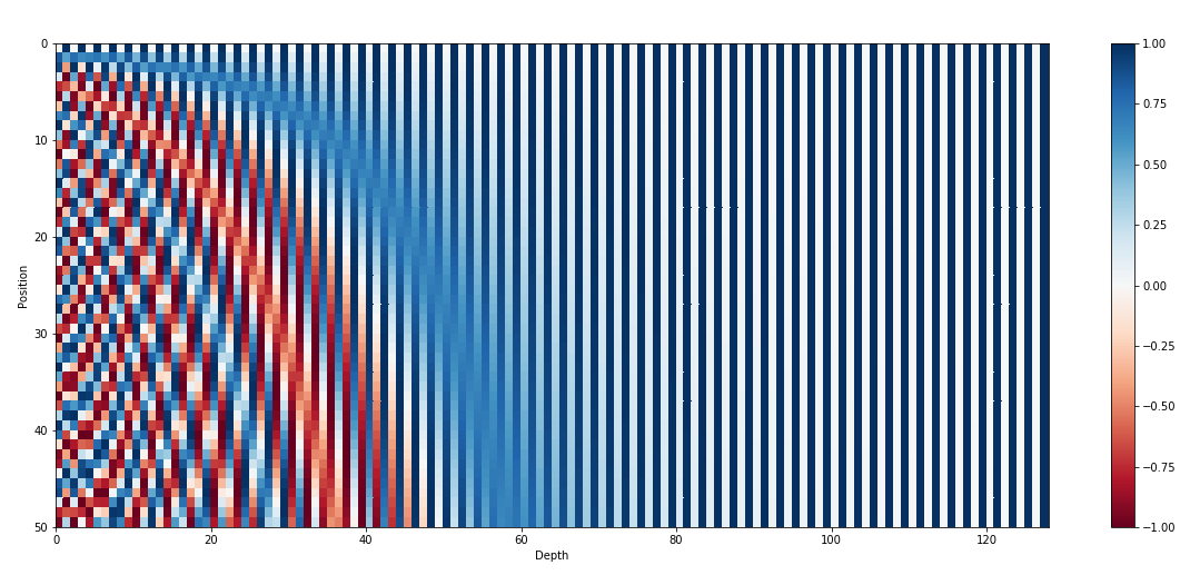
用更加科学的话来说，就是越靠后的位置波长越长、频率越低，位置越靠前频率越高。

二、相对性。存在一个和 $t$ 无关的线性变换，记为矩阵 $M$，能够满足：

\[\begin{array}{c} M.\begin{bmatrix} \sin(\omega_k . t) \\ \cos(\omega_k . t) \end{bmatrix} = \begin{bmatrix} \sin(\omega_k . (t + \phi)) \\ \cos(\omega_k . (t + \phi)) \end{bmatrix} \end{array}\]

这个矩阵是：

\[\begin{array}{c} M_{\phi,k} = \begin{bmatrix} \cos(\omega_k .\phi) & \sin(\omega_k .\phi) \\ - \sin(\omega_k . \phi) & \cos(\omega_k .\phi) \end{bmatrix} \end{array}\]

可以看仅仅和要变化的角度和位置向量中的位置有关系，和 token 位置没有关系：如果距离一定，那么 $\phi$ 可以固定下来，那么这个仅仅和位置 $k$ 有关系了；因此我们可以说每两个位置 $t$ 的位置向量都变换了一个固定的角度。也就满足了我们上面的要求 2。

三、距离对称性：token $t$ 和 token $k$ 的距离 == token $k$ 到 token $t$ 的距离。

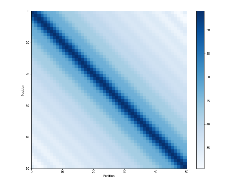
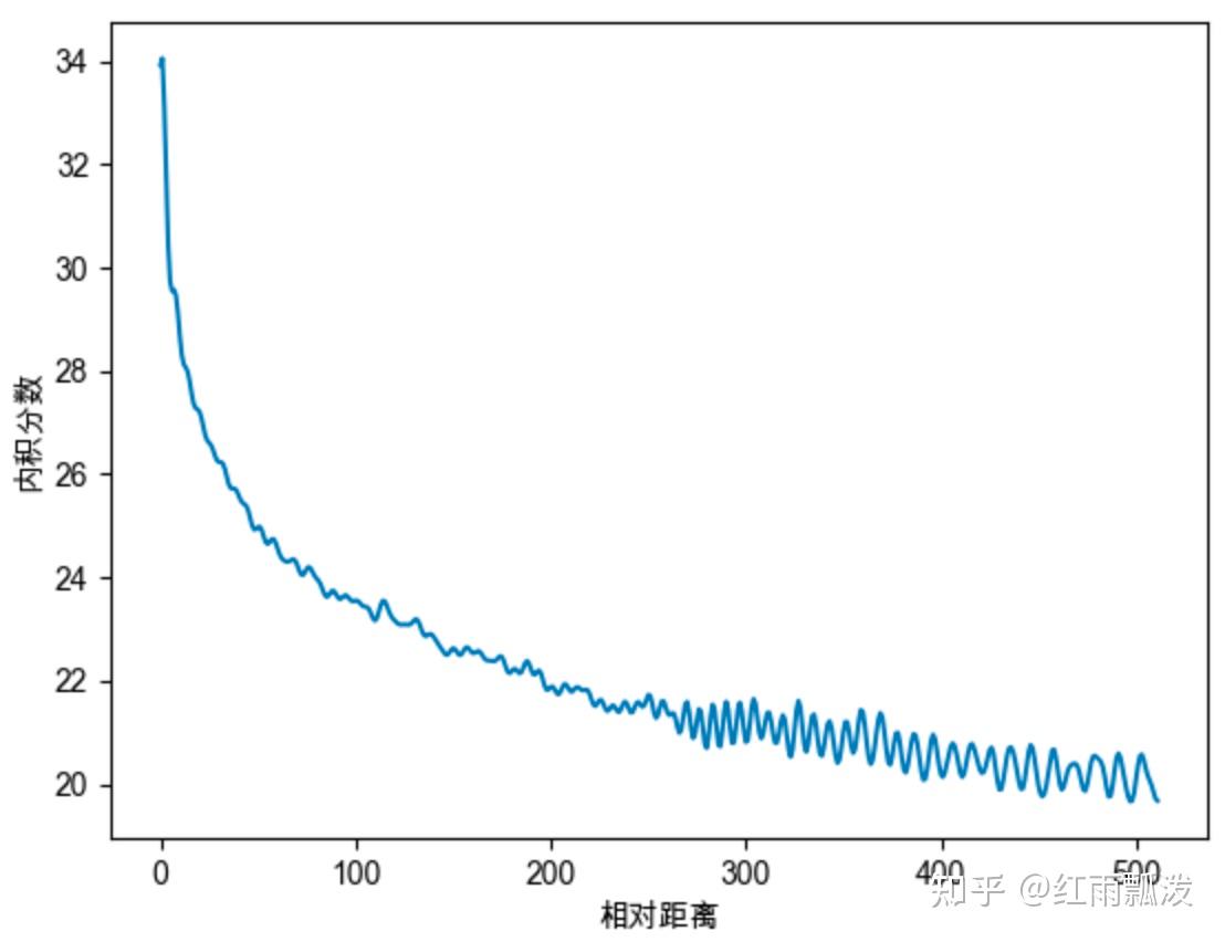
四、远程衰减性：距离越近，则他们的位置向量内积分数越高，反之则越低。不需要记住为什么远程衰减性为什么重要，只需要记住其和大模型的外推性有关系（也就是学的都是一定长度的 token，用的时候反而更长了）。

下面这个是位置向量的点乘，可见距离越远，越不相关，因为点乘值越小，也就越正交。

为什么不是直接 append 到 embedding 后面，而是直接加到词向量上？

一个可能的原因，这样更加节省参数量。

旋转位置编码 RoPE

加了位置信息的 token 的 $q$ 和 $k$ 为：$q_m = f(q,m)$, $k_m = f(k, m)$，$m$ 表示 token 位置，那么，我们希望 attention 信息中能有两个 token 之间的相对位置信息，即：

\[q_m \cdot k_n = g(q,k,m-n)\]

我们有一个参数和位置 $m$ 有关的旋转矩阵 $R_m$，在我们的 token 嵌入向量转换成 $q$, $k$ 向量之后，可以进一步给 $q, k$ 加入位置信息。这个矩阵有以下性质（怎么推导暂时不表）：

\[q_m \cdot k_n = (R_m q)^T \times (R_nk) = q^T R_{n-m} k\]

这个编码的好处是，对于位置信息的编码完全取决于 $n-m$，而不是取决于 $n$ 或者是 $m$ 的绝对值。也就是位置 0 到位置 1 与位置 50 到 51 的距离是一样的。$R_m$ 也有一个参数 $\theta$，可以用来调整每次旋转的角度的大小，这个其实不难想象。

在多维空间下，角度当然也是可以拆分的。

更详细的还是看这篇参考资料：(11 封私信 / 80 条消息) 图解RoPE旋转位置编码及其特性 - 知乎 只需要知道最后的计算方法是：

\[\begin{array}{c} \left(\begin{array}{c}q_0 \\ q_1 \\ q_2 \\ q_3 \\ \vdots \\ q_{d-2} \\ q_{d-1}\end{array}\right) \otimes\left(\begin{array}{c}\cos m \theta_0 \\ \cos m \theta_0 \\ \cos m \theta_1 \\ \cos m \theta_1 \\ \vdots \\ \cos m \theta_{d / 2-1} \\ \cos m \theta_{d / 2-1}\end{array}\right)+\left(\begin{array}{c}-q_1 \\ q_0 \\ -q_3 \\ q_2 \\ \vdots \\ -q_{d-1} \\ q_{d-2}\end{array}\right) \otimes\left(\begin{array}{c}\sin m \theta_0 \\ \sin m \theta_0 \\ \sin m \theta_1 \\ \sin m \theta_1 \\ \vdots \\ \sin m \theta_{d / 2-1} \\ \sin m \theta_{d / 2-1}\end{array}\right)\\ \end{array}\]

我们需要计算拿到的编码向量其实就是 $cos$ 向量和 $sin$ 向量。计算的时候使用 $Q$ 矩阵及改之后的 $Q$ 矩阵来分别乘以这两个向量并相加即可。

看一下实现吧：

# 这里实现了纯文本的和多模态的支持，取决于 Positions 这个向量的形状
# Query 和 key 的形状可以看出来，是 multihead attention
# Query 就是 Q 矩阵，key 就是 K 矩阵
@torch.compile(dynamic=True)
def forward(
    self,
    positions: torch.Tensor,
    query: torch.Tensor,
    key: torch.Tensor,
) -> Tuple[torch.Tensor, torch.Tensor]:
    """PyTorch-native implementation equivalent to forward().

    Args:
        positions:
            [num_tokens,] (text only) or
            [3, num_tokens] (T/H/W positions with multimodal inputs)
        query: [num_tokens, num_heads * head_size]
        key: [num_tokens, num_kv_heads * head_size]
    """
    assert positions.ndim == 1 or positions.ndim == 2
    num_tokens = positions.shape[-1]
    
    #上面的 sin 和 cos 两个向量，因为仅仅和位置有关系，所以我们缓存起来
    cos_sin = self.cos_sin_cache[positions]
    #cos sin 分成两个 tensor
    cos, sin = cos_sin.chunk(2, dim=-1)
    #mrope，我们暂时先忽略这块
    if positions.ndim == 2:
        assert self.mrope_section

        cos = torch.cat(
            [m[i] for i, m in enumerate(cos.split(self.mrope_section, dim=-1))],
            dim=-1,
        )
        sin = torch.cat(
            [m[i] for i, m in enumerate(sin.split(self.mrope_section, dim=-1))],
            dim=-1,
        )

    query_shape = query.shape
    #head_size 表示每一个 head 的列数，把 Q 矩阵按照 MHA 的方式，也就是沿着列的维度进行拆分。
    #按照 head_size 拆成 n 个 head。query 这个 tensor 从 2 维变成了 3 维。
    query = query.view(num_tokens, -1, self.head_size)
    #self.rotary_dim 是一个
    query_rot = query[..., : self.rotary_dim]
    query_pass = query[..., self.rotary_dim :]
    #计算得到加入了 rotary_embedding 信息之后的 query
    query_rot = _apply_rotary_emb(query_rot, cos, sin, self.is_neox_style)
    #
    query = torch.cat((query_rot, query_pass), dim=-1).reshape(query_shape)

    key_shape = key.shape
    key = key.view(num_tokens, -1, self.head_size)
    key_rot = key[..., : self.rotary_dim]
    key_pass = key[..., self.rotary_dim :]
    key_rot = _apply_rotary_emb(key_rot, cos, sin, self.is_neox_style)
    key = torch.cat((key_rot, key_pass), dim=-1).reshape(key_shape)
    return query, key
    
def _apply_rotary_emb(
    x: torch.Tensor,
    cos: torch.Tensor,
    sin: torch.Tensor,
    is_neox_style: bool,
) -> torch.Tensor:
    """
    Args:
        x: [num_tokens, num_heads, head_size]
        cos: [num_tokens, head_size // 2]
        sin: [num_tokens, head_size // 2]
        is_neox_style: Whether to use the Neox-style or GPT-J-style rotary
            positional embeddings.
    """
    #给倒数第二列加一个维度
    #[num_tokens, 1, head_size // 2]
    cos = cos.unsqueeze(-2).to(x.dtype)
    #给倒数第二列加一个维度
    #[num_tokens, 1, head_size // 2]
    sin = sin.unsqueeze(-2).to(x.dtype)
    if is_neox_style:
        x1, x2 = torch.chunk(x, 2, dim=-1)
    else:
        #下面两行表示把 x 按照最后一列分成了两部分。
        #表示在最后一维上，每隔 2 个取 1 个元素，从 索引 0 开始。
        x1 = x[..., ::2]
        #表示在最后一维上，从索引 1 开始，每隔 2 个取 1 个。
        x2 = x[..., 1::2]
    #非常好理解，看上面的最终的矩阵乘公式就行了。
    o1 = x1 * cos - x2 * sin
    o2 = x2 * cos + x1 * sin
    if is_neox_style:
        return torch.cat((o1, o2), dim=-1)
    else:
        #首先按元素堆叠，也就是把上面的计算结果聚合起来
        #堆叠完之后是 [[1, 2], [3, 4]...] 的状态，因此需要 flatten 来展平
        return torch.stack((o1, o2), dim=-1).flatten(-2)

一些思考：

• 当 $\theta$ 固定后，两个编码向量仅仅和 $m$ 也就是 token 的位置有关系。我们可以为每一个位置提前计算出来这两个向量，在每轮对话的时候复用这两个向量就好了。
• RoPE 相比于原来的编码（或者叫Sinusoidal 位置编码），区别在于 RoPE 不是直接计算一个向量加上原来的 embedding 向量上了。而是直接用一个函数来对 $q, k$ 向量来计算 $q_m = f(q, m)$。

M-RoPE

多模态场景下的 RoPE。

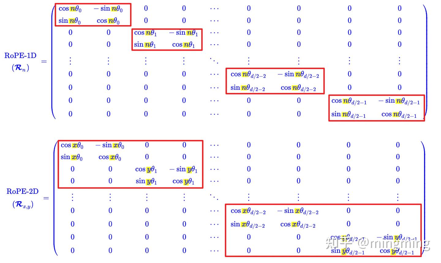
M-ROPE 通过将原始旋转嵌入分解为代表时间、高度和宽度的三个部分，使得大规模语言模型能够同时捕捉和整合一维文本序列、二维视觉图像以及三维视频的位置信息。

• 文本使用了第一维，也就是时间，矩阵是两两一组，位置用 $n$ 来表示；
• 图像使用了二三维，也就是高度和宽度，矩阵是四四一组，位置用 $(x,y)$ 来表示；
• 视频使用了一二三维，也就是时间高度和宽度，矩阵是六六一组，位置用 $(n,x,y)$ 来表示。

从计算上来说的区别：

注意下面公式每四行是一组： $$

\begin{array}{c} \left(\begin{array}{c}q_0 \ q_1 \ q_2 \ q_3 \ \vdots \ q_{d-4} \ q_{d-3} \ q_{d-2} \ q_{d-1}\end{array}\right) \otimes\left(\begin{array}{c} \cos x \theta_0 \ \cos x \theta_0 \ \cos y \theta_1 \ \cos y \theta_1 \ \vdots \ \cos x \theta_{d / 2-2} \ \cos x \theta_{d / 2-2} \ \cos y \theta_{d / 2-1} \ \cos y \theta_{d / 2-1}\end{array}\right)+\left(\begin{array}{c}-q_1 \ q_0 \ -q_3 \ q_2 \ \vdots \ -q_{d-3} \ q_{d-4} \ -q_{d-1} \ q_{d-2}\end{array}\right) \otimes\left(\begin{array}{c}\sin x \theta_0 \ \sin x \theta_0 \ \sin y \theta_1 \ \sin y \theta_1 \ \vdots \ \sin x \theta_{d / 2-2} \ \sin x \theta_{d / 2-2} \ \sin y \theta_{d / 2-1} \ \sin y \theta_{d / 2-1}\end{array}\right)\ \end{array}

$$ 单从计算上来说，并不会增加更多的计算量。$q$ 矩阵不用变，唯一需要变的就是 $cos$ 和 $sin$ 的这两个向量。

下面看 SGLang 里的代码：

# 这里实现了纯文本的和多模态的支持，取决于 Positions 这个向量的形状
# Query 和 key 的形状可以看出来，是 multihead attention
# Query 就是 Q 矩阵，key 就是 K 矩阵
@torch.compile(dynamic=True)
def forward(
    self,
    positions: torch.Tensor,
    query: torch.Tensor,
    key: torch.Tensor,
) -> Tuple[torch.Tensor, torch.Tensor]:
    """PyTorch-native implementation equivalent to forward().

    Args:
        positions:
            [num_tokens,] (text only) or
            [3, num_tokens] (T/H/W positions with multimodal inputs)
        query: [num_tokens, num_heads * head_size]
        key: [num_tokens, num_kv_heads * head_size]
    """
    assert positions.ndim == 1 or positions.ndim == 2
    num_tokens = positions.shape[-1]
    
    #上面的 sin 和 cos 两个向量，因为仅仅和位置有关系，所以我们缓存起来
    cos_sin = self.cos_sin_cache[positions]
    #cos sin 分成两个 tensor
    cos, sin = cos_sin.chunk(2, dim=-1)
    #mrope
    if positions.ndim == 2:
        #这是一个
        assert self.mrope_section

        #根据 sections 计算上面的两个向量
        cos = torch.cat(
            [m[i] for i, m in enumerate(cos.split(self.mrope_section, dim=-1))],
            dim=-1,
        )
        #根据 sections 计算上面的两个向量
        sin = torch.cat(
            [m[i] for i, m in enumerate(sin.split(self.mrope_section, dim=-1))],
            dim=-1,
        )

    query_shape = query.shape
    #head_size 表示每一个 head 的列数，把 Q 矩阵按照 MHA 的方式，也就是沿着列的维度进行拆分。
    #按照 head_size 拆成 n 个 head。query 这个 tensor 从 2 维变成了 3 维。
    query = query.view(num_tokens, -1, self.head_size)
    #self.rotary_dim 是一个
    query_rot = query[..., : self.rotary_dim]
    query_pass = query[..., self.rotary_dim :]
    #计算得到加入了 rotary_embedding 信息之后的 query
    query_rot = _apply_rotary_emb(query_rot, cos, sin, self.is_neox_style)
    #
    query = torch.cat((query_rot, query_pass), dim=-1).reshape(query_shape)

    key_shape = key.shape
    key = key.view(num_tokens, -1, self.head_size)
    key_rot = key[..., : self.rotary_dim]
    key_pass = key[..., self.rotary_dim :]
    key_rot = _apply_rotary_emb(key_rot, cos, sin, self.is_neox_style)
    key = torch.cat((key_rot, key_pass), dim=-1).reshape(key_shape)
    return query, key
    
def _apply_rotary_emb(
    x: torch.Tensor,
    cos: torch.Tensor,
    sin: torch.Tensor,
    is_neox_style: bool,
) -> torch.Tensor:
    """
    Args:
        x: [num_tokens, num_heads, head_size]
        cos: [num_tokens, head_size // 2]
        sin: [num_tokens, head_size // 2]
        is_neox_style: Whether to use the Neox-style or GPT-J-style rotary
            positional embeddings.
    """
    #给倒数第二列加一个维度
    #[num_tokens, 1, head_size // 2]
    cos = cos.unsqueeze(-2).to(x.dtype)
    #给倒数第二列加一个维度
    #[num_tokens, 1, head_size // 2]
    sin = sin.unsqueeze(-2).to(x.dtype)
    if is_neox_style:
        x1, x2 = torch.chunk(x, 2, dim=-1)
    else:
        #下面两行表示把 x 按照最后一列分成了两部分。
        #表示在最后一维上，每隔 2 个取 1 个元素，从 索引 0 开始。
        x1 = x[..., ::2]
        #表示在最后一维上，从索引 1 开始，每隔 2 个取 1 个。
        x2 = x[..., 1::2]
    #非常好理解，看上面的最终的矩阵乘公式就行了。
    o1 = x1 * cos - x2 * sin
    o2 = x2 * cos + x1 * sin
    if is_neox_style:
        return torch.cat((o1, o2), dim=-1)
    else:
        #首先按元素堆叠，也就是把上面的计算结果聚合起来
        #堆叠完之后是 [[1, 2], [3, 4]...] 的状态，因此需要 flatten 来展平
        return torch.stack((o1, o2), dim=-1).flatten(-2)

参考资料：

- (5 封私信 / 80 条消息) Qwen2-VL技术解析（二）- M-ROPE - 知乎